In this article we are going to discuss the third and last equation motion. Like previous two equations, this also has very much of applications in the field of mechanics. So let’s learn this equation also with the help of graphical method.
Consider the body moving in XY plane starts its motion from point P with initial velocity ‘u’ (u ≠ 0) and reaches to point Q in time ‘t’ with uniform acceleration ‘a’ and final velocity ‘v’ shown in figure below.
In graph X- axis represents time and Y-axis represents velocity,

From graph we have,
OP=u (initial velocity)
OQ’=v (final velocity)
OS=t (time)
Draw QS perpendicular to X axis
Now draw PR ll OS
Then from graph, OS=PR,OP=SR and
OQ’ – OP = RQ = v – u = change in velocity
Third equation of motion:
Third equation of motion can be obtained by slight modification in mathematical steps used in derivation of second equation. Here also according to definition of velocity, distance covered by object is nothing but the area of quadrilateral OPQS. Here we are going to just use the formula for trapezium since quadrilateral OPQS acts as trapezium if the entire diagram is rotated by 900 in clockwise sense.
∴ displacement or distance covered = area of trapezium OPQS

For more illustration of the 3rd equation, just go through the following numerical,
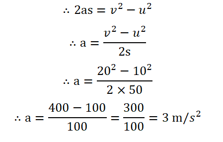
1.) Car covers the distance of 50 m, when it changes its speed from 36 km/hr to 72 km/hr. What is the acceleration of car?
Ans: Here, u= 36 km/hr=10 m/s
v= 72 km/hr=20 m/s
s= 50 m
From 3rd equation of motion,